robustGMM fits univariate Gaussian mixture models when the data may be contaminated by outliers. It provides three EM-type fitters with a common interface, plus a data-driven rule for choosing the robustness tuning parameter:
-
robustGMM()— the density power (beta-)divergence estimator of Fujisawa and Eguchi (2006).beta = 0recovers maximum likelihood; largerbetadown-weights observations that are implausible under the fitted mixture. -
uniformNoiseGMM()— a Gaussian mixture with an additional uniform “noise” component (as inmclust’s noise model). The posterior probability of the noise component is a natural outlier score for each observation. -
vanillaGMM()— the standard maximum likelihood EM baseline. -
loo_cvm_div()— leave-one-out Cramér–von Mises divergence for selectingbeta.
The fitters are validated against established implementations: vanillaGMM() against mixtools::normalmixEM() and uniformNoiseGMM() against mclust’s noise-component model.
Installation
You can install the development version of robustGMM from GitHub with:
# install.packages("devtools")
devtools::install_github("ge-li/robustGMM")
Example
Draw a two-component mixture and contaminate it with an outlier:
library(robustGMM)
set.seed(404)
lambda <- c(0.25, 0.75)
mu <- c(0, 4)
sigma <- c(1, 1)
x <- rnormix(n = 100, lambda, mu, sigma)
x[which.max(x)] <- 10 # outlier
plot(density(x))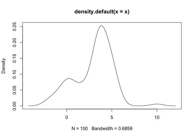
plot of chunk unnamed-chunk-2
The outlier inflates the scale estimate of the maximum likelihood fit:
mle <- vanillaGMM(x, lambda, mu, sigma)
rbind(mu = mle$mu, sigma = mle$sigma)
#>             [,1]     [,2]
#> mu    -0.1283825 3.906790
#> sigma  1.0038883 1.244058
The robust fit resists it:
rob <- robustGMM(x, lambda, mu, sigma, beta = 0.1)
rbind(mu = rob$mu, sigma = rob$sigma)
#>            [,1]      [,2]
#> mu    0.1430803 3.9728562
#> sigma 1.1657071 0.9474814
All fitters report convergence honestly: if maxiter is reached, the last iterate is returned with converged = FALSE and a warning, never a silent NULL.
Modeling outliers explicitly
uniformNoiseGMM() adds a uniform component over the data range, and the posterior probability of that component scores each observation as an outlier:
noise_fit <- uniformNoiseGMM(x, lambda * 0.98, mu, sigma, lambda0 = 0.02)
gauss_part <- noise_fit$lambda[1] * dnorm(x, noise_fit$mu[1], noise_fit$sigma[1]) +
  noise_fit$lambda[2] * dnorm(x, noise_fit$mu[2], noise_fit$sigma[2])
post_noise <- (noise_fit$lambda0 / noise_fit$V) /
  (noise_fit$lambda0 / noise_fit$V + gauss_part)
which(post_noise > 0.5) # flags the planted outlier
#> [1] 41
Selecting the tuning parameter
loo_cvm_div() computes a leave-one-out Cramér–von Mises divergence between the data and the fitted model; pick the beta that minimizes it:
betas <- seq(0.01, 0.2, by = 0.01)
div <- vapply(betas, function(b) loo_cvm_div(x, lambda, mu, sigma, b), numeric(1))
plot(betas, div, xlab = "beta", ylab = "LOO Cramér–von Mises divergence",
     main = "Tuning parameter selection on contaminated data")
abline(v = betas[which.min(div)], col = "darkgreen", lty = 2)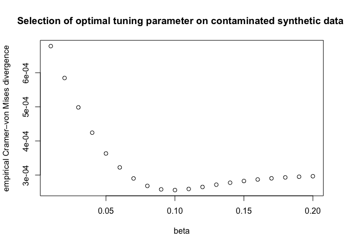
plot of chunk unnamed-chunk-6
A note on robustness and initialization
Robustness of the beta-divergence estimator is a property of the local optimum: the EM algorithm down-weights points that are implausible under the current fit. If the initialization places a component on a tight cluster of outliers, every EM variant — robust or not — will happily keep it there, and with the number of components fixed, no global fit criterion identifies the “typical” model. In practice, initialize from a contamination-resistant summary of the data (for example, quantiles of a trimmed sample) rather than from raw k-means centers.